Note to reader
This was an assignment for my ML class at Northwestern, and while I do include the code in this, I want to be clear that this is my group’s work and should not be used for any future assignments.
Github Link
- Private url
Overview
This assignment was a stepping stone in my interest in machine learning. We were given multiple datasets to work with based on a few different distributions that I would have to learn from using a neural network. We first had to implement a PyTorch simple neural network to solve the problem(s), and once we understood what the expected solutions should look similar to, we had to implement our solutions completely from scratch.
In doing so, I more clearly understood the math that was working within a neural network. It both debunked any fear on the subject and ignited a passion for the subject.
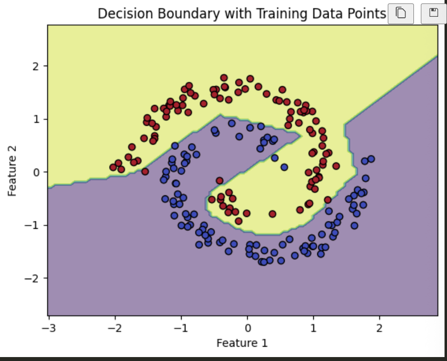
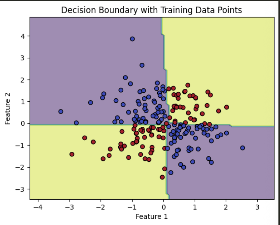
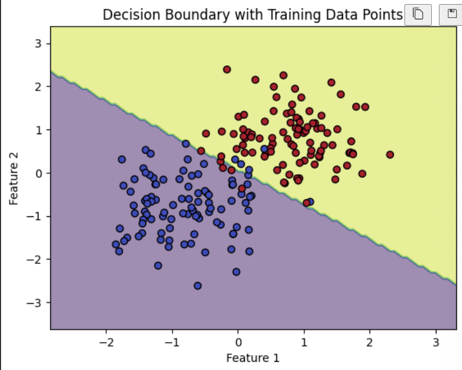
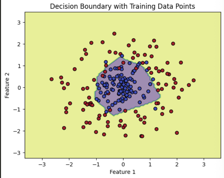
The dataset distributions that we needed to learn decision boundaries for were (also illustrated below):
- XOR
- Spiral
- Gaussian
- Center surround
PyTorch Implementation
Part one of this assignment was to utilize PyTorch to simply create a FFNN that could create the decision bounadies that are illustrated above.
Because this is an assignment that future students are likely to replicate, I will only include a few PyTorch snippets to get an idea of how this solution worked.
#
# Model architecture
#
class SimpleNN(torch.nn.Module):
    def __init__(self, input_size, hidden_size, output_size):
        super().__init__()
        self.f1 = torch.nn.Linear(input_size, hidden_size)
        self.relu = torch.nn.ReLU()
        self.f2 = torch.nn.Linear(hidden_size, output_size)

    def forward(self, x):
        x = self.f1(x)
        x = self.relu(x)
        x = self.f2(x)
        return x

#
# Training the model
#

def train(model, train_loader, valid_loader, num_epochs, criterion, optimizer):
    """
    Parameters
    ----------
    model: Pytorch nn.Module model
    train_loader: training set as a DataLoader()
    valid_loader: validation set as a DataLoader()
    num_epochs: Number of epochs
    criterion: Loss function
    optimizer: Optimization function
    """

    train_losses = []
    valid_losses = []

    for epoch in range(num_epochs):
        model.train()
        running_train_loss = 0.0

        for features, labels in train_loader:
            # Zero out gradients
            optimizer.zero_grad()

            # Predictions
            outputs = model(features)

            # Calculating the loss
            loss = criterion(outputs, labels)

            # Backprop
            loss.backward()

            # Updating parameters
            optimizer.step()

            # For analysis, we keep track of loss per batch
            running_train_loss += loss.item()

        epoch_train_loss = running_train_loss / len(train_loader)
        train_losses.append(epoch_train_loss)

        #
        # Validation set
        #
        model.eval()
        running_valid_loss = 0.0
        with torch.no_grad():
            for features, labels in valid_loader:
                outputs = model(features)
                loss = criterion(outputs, labels)

                running_valid_loss += loss.item()

        epoch_valid_loss = running_valid_loss / len(valid_loader)
        valid_losses.append(epoch_valid_loss)

        if (epoch + 1) % 50 == 0:
            print(f"Epoch {epoch+1}/{num_epochs}, Train Loss: {epoch_train_loss:.4f}, Valid Loss: {epoch_valid_loss:.4f}")

    return train_losses, valid_losses
PyTorch Results
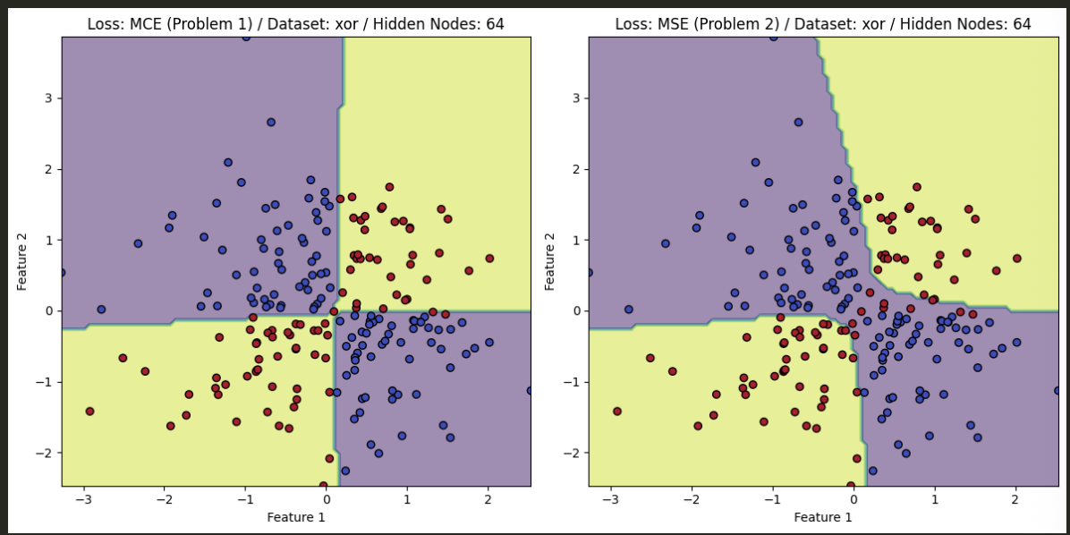
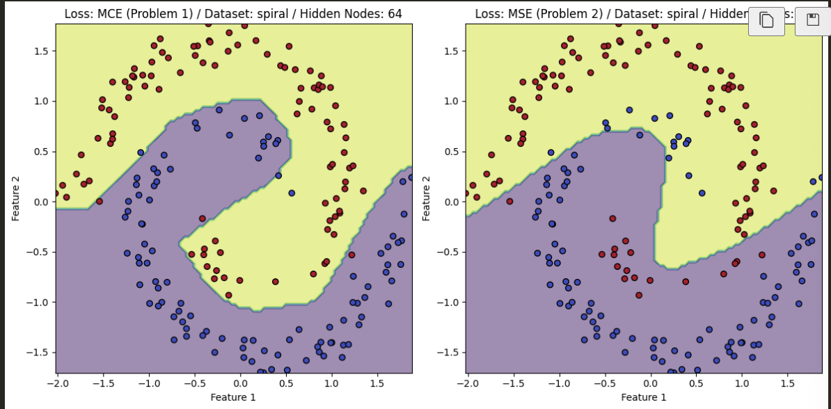
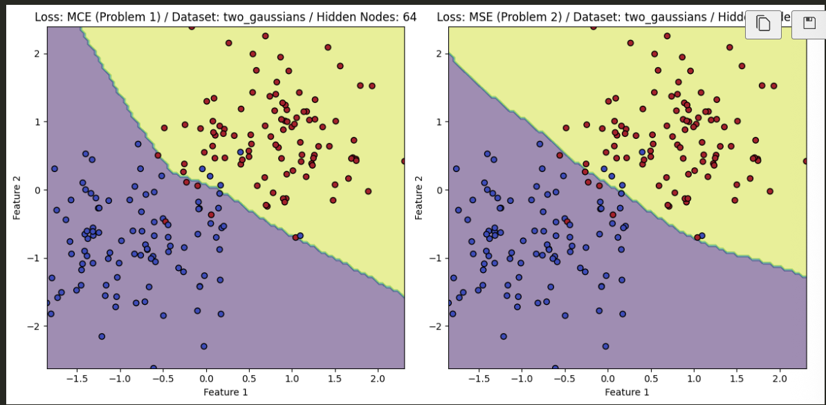
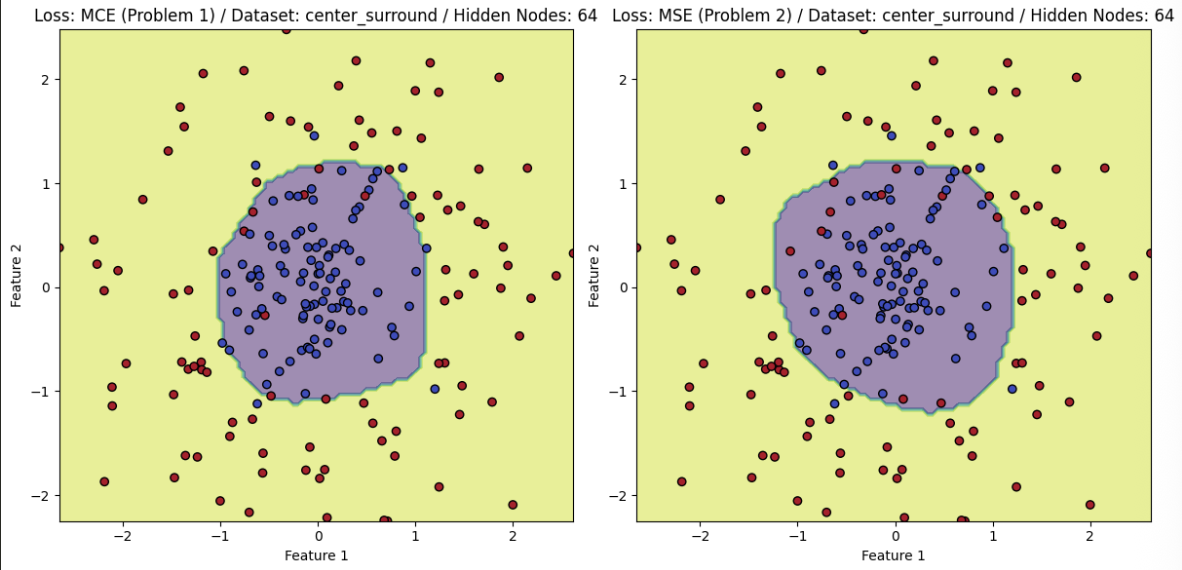
- The PyTorch results, after training, are found below and compare the difference between utilizing MSE and MCE for the task at hand.
XOR
Spiral
Gaussian
Center Surround
FFNN from Scratch
When implementing the NN from scratch, the first things that we had to accomplish was create the helper functions that were needed for calculating activations, as well as the derivatives of the functions.
Conceptual explaination
For those who may be reading this and have 0 experience with neural networks, we need to use derivatives to properly calculate our backpropogation. The forward pass of the model (moving left to right) calculates a final prediction for what the solution should be given the data at hand. Once we have the prediction, we calculate the loss (how off the mark and/ or accurate we are compared to our expected output), and then we backpropogate to learn by how much to adjust the internal values of our neural network. So at first, our neural network contains weights and biases that are unlearned semi-random values, after each step, though, we update these parameters to help minimize the loss (minimize how many mistakes we make in our calculations), but taking the derivative of the loss function with respect to the paramaters within the model. All this means, is that we take the derivatives (calculus) to see by how much to adjust each of the weights within the network so that the model can perform better (hopefully) on the next iteration. I don’t expect this to have taught you neural networks, but I hope it was somewhat helpful to reframe it maybe a little bit differently for any newcomers.
Helper functions
Anyways, the helper functions that we use for these calculations exist here:
def z_score(df, scaler):
    """
    Parameters
    ----------
    df: pd.DataFrame with labels in the first column and features in following columns
    scaler: sklearn.preprocessing.StandardScaler fit to the training dataset feature values

    Returns
    -------
    tuple: np.array of scaled features and np.array of labels
    """
    features = df.iloc[:, 1:]
    labels = df.iloc[:, 0].values

    features = scaler.transform(features)

    indices_order = np.random.permutation(len(features))

    features = features[indices_order]
    labels = labels[indices_order]

    return features, labels


def label_encoder(labels):
    """
    Parameters
    ----------
    labels: np.array of training dataset labels

    Returns
    -------
    dict: with one-hot encoded "numerical encoding: label" key: value pairs
    """
    unique_labels = sorted(np.unique(labels))
    labels_encoding = {i: l for i, l in enumerate(unique_labels)}
    return labels_encoding

def encode_labels(labels, encoder):
    """
    Parameters
    ----------
    labels: np.array of training dataset labels
    encoder : dict with "numerical encoding: label" key: value pairs

    Returns
    -------
    np.array of encoded labels
    """
    return np.array([encoder[l] for l in labels])

def decode_labels(encoded_labels, encoder):
    """
    Parameters
    ----------
    encoded_labels: np.array of encoded labels
    encoder: dict with "numerical encoding: label" key: value pairs

    Returns
    -------
    np.array: of decoded labels
    """
    decoder = {value: key for key, value in encoder.items()}
    return np.array([decoder[l] for l in encoded_labels])

def encoded_labels_array(encoded_labels):
    """
    Parameters
    ----------
    encoded_labels: np.array of encoded labels

    Returns
    -------
    np.array of encoded labels as arrays (e.g., encoded label 1 becomes [0, 1] and encoded label 0 becomes [1, 0])
    """
    num_unique_labels = len(np.unique(encoded_labels))
    return np.array([np.array([1 if i == el else 0 for i in range(num_unique_labels)]) for el in encoded_labels])

def softmax(logits):
    """
    Parameters
    ----------
    logits: np.array of logits (raw output from output layer)

    Returns
    -------
    np.array: of values after performing softmax (values sum to 1)
    """
    exp_logits = np.exp(logits - np.max(logits, axis=1, keepdims=True))
    return exp_logits / np.sum(exp_logits, axis=1, keepdims=True)

def mcce(softmax_logits, labels):
    """
    Parameters
    ----------
    softmax_logits: np.array of softmaxed logits (class probabilities)
    labels: np.array of true labels

    Returns
    -------
    np.float64: Multi-class cross entropy loss
    """
    return - np.sum(labels * np.log(softmax_logits)) / labels.shape[0]

def sigmoid(unactivated):
    """
    Parameters
    ----------
    unactivated: np.array of unactivated input matrix (output matrix from last layer @ weights)

    Returns
    -------
    np.array: Matrix after performing sigmoid operation on unactivated input matrix
    """
    return 1 / (1 + np.exp(-unactivated))

def sigmoid_derivative(activated):
    """
    Parameters
    ----------
    activated: np.array of activated input matrix

    Returns
    -------
    np.array: Matrix after performing sigmoid derivative operation on activated input matrix
    """
    return sigmoid(activated) * (1 - sigmoid(activated))

def relu(unactivated):
    """
    Parameters
    ----------
    unactivated: np.array of unactivated input matrix (output matrix from last layer @ weights)

    Returns
    -------
    np.array: Matrix after performing relu operation on unactivated input matrix
    """
    return np.maximum(0, unactivated)

def relu_derivative(activated):
    """
    Parameters
    ----------
    activated : np.array of activated input matrix

    Returns
    -------
    np.array: Matrix after performing relu derivative operation on activated input matrix
    """
    return (activated > 0).astype(float)
Forward pass
We decided that it would be best to create a model architecture that is similar to that of the PyTorch implementation. Therefore, our forward pass consists of a fully connected layer between the inputs and the first hidden layer, then we add the bias term, then we use the relu activation function to get the output of the first hidden layer.
Next we have another fully connected layer between the results from the first hidden layer and the weights of the second hidden layer, again add the bias terms, and then take the softmax activation function. The softmax function is used here to create a probability distribution of our predictions, and we will then use this vector of percentages that add up to 1, to take our prediction.
The forward pass (the shapes between the input to first hidden layer and the hidden layer to the output layer are not shown, but exist in shape_i_h, shape_h_o):
def forward(self, features, train=False):
    """
    Parameters
    ----------
    features: np.array of examples with each example being an array of feature values
    train : Optional[bool] - True if training the network (i.e., if intermediate results are needed to compute gradients), by default False

    Returns
    -------
    np.array: of outputs for each example with each output being an array of class probabilities
    """
    forward_results = {}

    forward_results['features'] = features
    i_h = features @ self.w_i_h
    forward_results['i_h'] = i_h
    i_h_b = i_h + self.b_i_h
    forward_results['i_h_b'] = i_h_b
    a_i_h_b = relu(i_h_b)
    forward_results['a_i_h_b'] = a_i_h_b

    h_o = a_i_h_b @ self.w_h_o
    forward_results['h_o'] = h_o
    h_o_b = h_o + self.b_h_o
    forward_results['h_o_b'] = h_o_b
    a_h_o_b = softmax(h_o_b)
    forward_results['a_h_o_b'] = a_h_o_b

    if train:
        return a_h_o_b, forward_results
    return a_h_o_b
Backward pass
This is where we have to calculate the derivative of the loss function with respect to the model paramters to learn by how much to adjust the model parameters to minimize the loss function. Also, for learning purposes, the derivative of the loss function with respect to the model paramters will calculate by how much to adjust the values to maximize the loss function we negate this to minimize it.
All calculations were done by hand outside of the code, and then later implemented based on our calculations.
def backward(self, forward_results, labels):
    """
    Parameters
    ----------
    forward_results: dict of all results (input, intermediates, and output) from forward a pass
    labels: np.array of encoded labels

    Returns
    -------
    dict: of gradient matrices of weight and bias matrices
    """
    gradients = {}

    probs = forward_results['a_h_o_b']

    dL_dh_o_b = probs - labels

    a_i_h_b = forward_results['a_i_h_b']
    gradients['w_h_o'] = a_i_h_b.T @ dL_dh_o_b
    gradients['b_h_o'] = np.sum(dL_dh_o_b, axis=0, keepdims=True)

    dL_da_i_h_b = dL_dh_o_b @ self.w_h_o.T
    dL_di_h_b = dL_da_i_h_b * relu_derivative(forward_results['a_i_h_b'])

    gradients['w_i_h'] = forward_results['features'].T @ dL_di_h_b
    gradients['b_i_h'] = np.sum(dL_di_h_b, axis=0, keepdims=True)

    return gradients
Updating the parameters
Now that we have backpropogated, we have a way to adjust the actual weights and biases within the model.
def update_weights(self, gradients, learning_rate):
    """
    Parameters
    ----------
    gradients: dict of gradient matrices of weight and bias matrices
    learning_rate: float that controls the size of the step taken during the update
    """
    self.w_h_o -= (learning_rate * gradients['w_h_o'])
    self.b_h_o -= (learning_rate * gradients['b_h_o'])
    self.w_i_h -= (learning_rate * gradients['w_i_h'])
    self.b_i_h -= (learning_rate * gradients['b_i_h'])
Training the model
Training the model works extremely similarly to the PyTorch implementation, it just uses our own helper functions that I have included above to go throught he forward pass, backward pass, and then how we should update our weights for the next iteration.
FFNN from Scratch Results
Spiral
XOR
Gaussian
Center Surround
Conclusion
This was an extremely fulfilling project because it taught me to be less afraid of the equations that exist within ML. And also, that the equations that we use all make very clear sense and can explain everything within the space. I apologize to anyone who is less familiar in the ML space, this page is not meant for beginners, it is only a summary for anyone interested in my work. I may in the future create a site on my portfolio that goes through all the steps needed to understand what is happening from scratch so that others may implement it on their own for fun!